Metrics explained: Classification and Tagging
Classification metrics
In classification set up, the classes are exclusive : prediction of multiple classes for the same image is not possible. Also predicting no class is not possible.
The predicted class is the one with maximum probability.
Confusion Matrix
For this example, we are still dealing with cars and bikes.
The dataset is this time balanced, and of 1000 images (500 bikes, 500 cars)
Here is the situation of the predictions presented in a confusion matrix
Car
420
110
Bike
80
390
The table above is called a confusion matrix.
Cars predicted as Cars, and Bikes predicted as Bikes constitute the good answers, the rest is confusions of bikes with cars and vice versa
True Positive, False positive, False negative, True negative
In general, talking about true positive, in the case of binary classification, we need to take a perspective of one of the two classes, for example cars.
Car is the positive class in this case, and bike the negative class (not a car)
True positive (TP) is a car that has been predicted as a car
False positive (FP) is a bike that has been predicted as a car
False negative (FN) is a car that has been predicted as a bike
True negative (TN) is a bike that has been predicted as a bike
Accuracy
Accuracy is simply the number of correct answers over the number of total answers
From this matrix we can compute the following metrics :
The accuracy of this model is 0.81 (81%)
Formal definition
Disclaimer
The value of accuracy can be misleading in case of unbalanced dataset.
Example
Hypothetically we have dataset of 100 images, of two classes ( cars and bikes), the number of images of class car is 95, the number of images of class bike is 5.
If we have a dumb model that predicts car no mater the image we gave it as an input, this model will have an accuracy of 95/100 = 0.95, which seems to be of high value, but the model is in fact useless.
Recall
Let us take the perspective of the class car
Recall can be understood as the proportion of accurately predicted cars to the actual number of cars (which is the sum of the first column)
In our example, this value will be
Recall_car = 420 / 500 = 0.84
Taking the perspective of bikes
Recall_bike = 390 / 500 = 0.78
This model has a higher recall of cars than bikes.
Formal definition
Precision
From the perspective of cars, precision can be understood intuitively as being the ratio of true cars when the model predict a car. In different words, the ratio of correct predictions of cars among the total number of predicted cars, which is the sum of the first row.
With numbers
Precision_car = 420 / 530 = 0.79
from the perspective of bikes
Precision_bike = 390/470 = 0.83
So this model has a higher precision in predicting bikes than cars
Formal definition
Tagging metrics
In tagging setup, an image can have a prediction from 0 to multiple classes.
The output of the model gives a probability for each class, in an independent way between classes. A choice of a threshold per class is then necessary to calibrate the model.
If the probability of a class is higher than its threshold, the class is considered as predicted.
Hence, the classification metrics cannot be used unless:
We chose a threshold per class
We analyse each class independently, and we transform the problem into a binary classification : this class being predicted or not.
To avoid the burden of choosing the set of thresholds, we use the metric of mean average precision.
Mean average precision
To define Mean Average Precision, we need to start by computing the Average Precision of each class, and then compute their average.
Formal definition
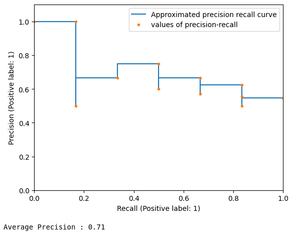
An approximation of this value is computed by changing the threshold, and computing the value of Precision at each value of threshold multiplied by the change of value of Recall (between the previous and the current value of threshold)
Example
In the case we want to evaluate the performance of a given model on a test set of 12 elements with the following ground truths and predictions
0
0.9
0
0.1
0
0.3
0
0.6
0
0.2
0
0.4
1
0.15
1
0.5
1
0.95
1
0.8
1
0.35
1
0.65
Changing the threshold from values of 0 to 1, the values of Recall and Precision changes
The different points on the graph highlight when either Recall or Precision changes value
At a threshold of value 0.15 we have a value of 1 and a precision of 6/11
At a threshold of value 0.5, the Recall is 4/6 = 0.667 and the Precision is also 4/6 = 0.667
Computing all the points and calculating the area under the interpolated Precision-Recall curve results in the value of Average Precision

In the case of multi-class tagging, we generalize this value, by computing the Average Precision of each class, then computing their mean, which results in the value of Mean Average Precision
Was this helpful?